Pyhsical disks are the inevitable backbone of data storage, no matter if spinning disks or flash storage. Unfortunately, physical disks will fail eventually, creating a need for redundant storage implementations to prevent data loss when disks die.
What is RAID?
RAID stands for Redundant Array of Independent Disks. It consists of multiple different configurations commonly called "RAID levels", each providing it's own balance of performance, storage space and redundancy. Depending on the chosen level, combining disks into RAID arrays can offer improved performance by spreading data evenly across disks, offer redundancy to survive disk failures or merge multiple physical disks into a single virtual disk to simplify data access for applications. Since the benefits for the added complexity and cost of RAID systems is largely useless to end users, RAID is mainly used in enterprise or dedicated storage systems like NAS devices or servers.
Hardware RAID vs Software RAID
Software RAID is implemented through the MD (Multiple Devices) kernel module in linux, and managed with the mdadm command-line utility. It is available by default in most linux systems and requires no special hardware or setup. While it comes at no cost, it needs CPU and RAM resources to manage RAID levels, thus lowering the overall system performance, and provides limited redundancy, since write caches are mostly kept in memory. A power outage may cause loss of data that was only kept in cache and not yet committed to disk. The overhead on system resources varies by RAID level; levels 0 and 1 typically incur negligible performance penalties, while levels 5 and 6 can place a noticeable strain on the CPU.
Hardware RAID uses a dedicated piece of hardware called a RAID controller, either built into the motherboard or as a separate card. Hardware RAID is typically controlled through the BIOS interface provided by the raid controller or special software from the hardware vendor. The hardware card will handle all RAID tasks, putting no additional strain on CPU/RAM resources, and often come with additional features like battery-backed caches to ensure writes are synced to disk even during power outages. Hardware RAID controllers can be quite expensive and can introduce a single point of failure to the system (if the RAID controller dies, all disks become inaccessible).
Linear RAID
A linear RAID setup simply combines multiple physical disks into one virtual disk, effectively merging their available space. It is similar to other JBOD (Just a Bunch Of Disks) configurations and provides no benefits in terms of performance or fault tolerance. it uses the underlying disks sequentially, filling the first disk in the array entirely before writing data to the next one. This allows a linear RAID configuration to be extended easily by appending empty disks to the array.The main use of this RAID level is to circumvent software issues, for example when a program uses a single directory to store large amounts of data, linear RAID allows administrators to mount multiple disks combined at a single directory mount point, making all their space available to the program.
RAID 0 (striping)
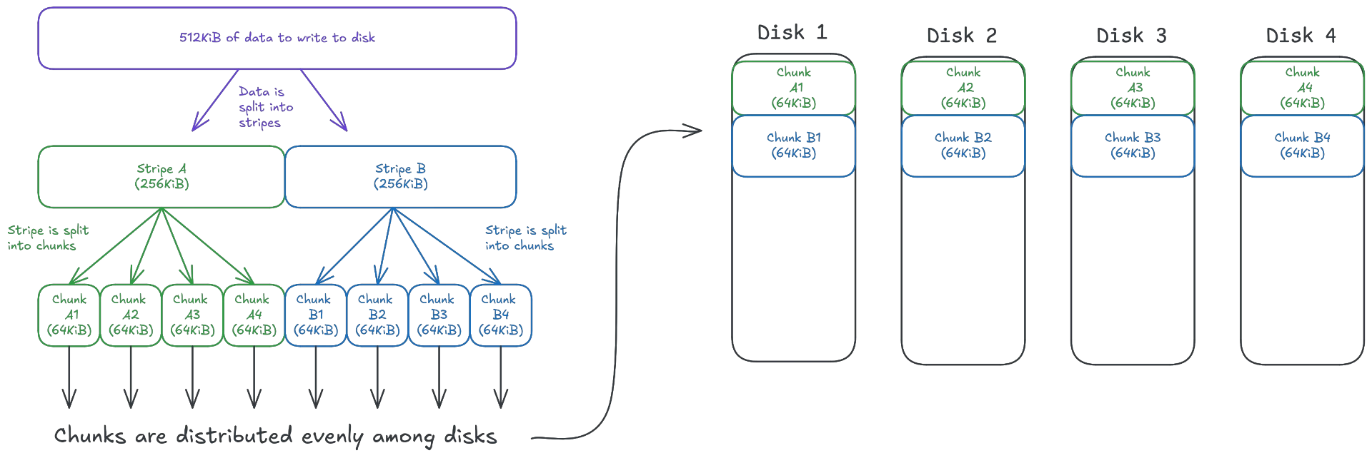
Striping is a mechanism by which data is split into chunks (stripes), and each stripe is written evenly across all disks in the array. A default configuration would use 64KiB per disk as a stripe size, resulting in 256KiB stripe size for an array with 4 disks. As a practical example, writing 512KiB of data to a striped RAID array with 4 disks would first split the data into stripes of 256KiB (64KiB * 4 disks), then split the stripes into 64KiB chunks, with each disk writing one chunk per stripe.
The main reason to use striping is performance: assuming a RAID 0 array has 4 disks with 1MB/s read performance per disk, a file striped among all 4 disks could potentially be read with up to 4MB/s, as each disk is involved in the reading process. The same benefits are observable for writes. Striping distributes the stored data (and their read/write operations) evenly among all available disks, aiming to use all available disk bandwidth capacity per disk.
While striping is a great way to spread data and filesystem load, it can be problematic for tiny read/write operations: a read or write will always involve the entire stripe the data is stored in. Assuming a stripe size of 256KiB, even a tiny read or write of 2 bytes would still need to read/write the entire 256KiB stripe to/from all disks in the array.
Striping offers no fault tolerance, but can greatly increase throughput speed for file operations, scaling linearly with the number of disks in the array (more disks = faster reads/writes).
RAID 1 (mirroring)
This RAID level is mainly intended for redundancy, with some performance benefits. Mirroring simply writes all data to two (or more) disks, enabling the system to seamlessly switch over to the mirror disk if the primary one fails. RAID 1 setups can survive disk failures at runtime without performance degradation, as long as a mirror for the failed disk is still operational. While mirroring typically uses a single mirror disk, it can use multiple mirrors at the same time, allowing for several disks to fail without bringing the system down.
Since the data is available on all physical mirror disks, it can be read from multiple disks at the same time, scaling read performance linearly with the number of disks in the array. Write performance is still limited by the slowest disk in the array, as data needs to be written to all disks.
Replacing a failed disk in a RAID 1 configuration will put a lot of load on the disk holding the data to sync to the new mirror (or vice versa). Using multiple mirror disks can help mitigate this issue, but will increase storage cost significantly.
The main downside of mirroring is cost: At most half of the available total storage space will be available to the system (as the other half is needed for mirroring data), further reduced when using more mirror disks.
RAID 10 (striped mirroring)
RAID 10 simply combines the benefits of RAID levels 0 and 1, storing data across all disks in stripes, while also mirroring all data. This approach brings both the benefits and downsides of RAID 0 and 1: read/write load is distributed evenly among all physical disks, the system survives a failing drive at runtime without any performance impact or data loss, but at most half of the total storage space is available to the system (further reduced with higher mirror counts).
Syncing data to a replacement for a failed disk may have different performance implications depending on the implementation: If the physical disks are organized as mirrored units (stripes written to RAID 1 units), then the syncing process behaves similarly to normal RAID 0, where the entire mirrored content is copied from the surviving disk. However, if the striped data is mirrored (where stripes or stripe chunks are mirrored across disks), then reads can be distributed among all disks during the syncing process, resulting in less overall load on each individual disk.
RAID 4 (striping with parity disk)
This configuration uses striping, but reserves a disk for parity data. Parity data is created by XORing the data of the data in all other disks. Should a disk become unavailable, the parity can be used to recompute the missing data (as long as no more than one disk is missing). Using a separate disk to store parity information enables administrators to add disks to the RAID array at runtime, without recomputing the parity information.
When recovering from a failing disk, this configuration puts significantly more load on the parity disk: While data needed to recompute the missing chunks is read from all disks, all parity writes go to the parity disk, potentially maxing out it's write capacity while recomputing data, reducing the overall array performance (as normal writes to other disks would also need to write updated parity data on the overloaded disk).
The biggest feature of striping with parity is the fact that it only requires a single disk for redundancy, making at least 66% of storage available (increasing with more disks; e.g. 5 disks would make 80% available etc). Parity requires at least 3 disks in the array and can recover from a single disk failure (but multiple failed disks at once will result in a fatal failure of the array).
Parity calculations cause some overhead, increasing with number of disks, which is why hardware RAID will perform better than software RAID for levels with parity.
RAID 5 (striped parity)
Improving on the idea of combining striping with parity data, RAID 5 goes one step further and splits the parity data itself into stripes, spreading it evenly across available disks among normal data. Since no single disk is dedicated to parity information, the load for recovering from a failed disk and parity writes is spread evenly across the array.
RAID 5 is one of the most popular configurations for common servers and backbone configurations, as it strikes a reasonable balance between fault-tolerance, performance and available storage.
RAID 6 (striped double parity)
RAID 6 adds more fault tolerance on top of RAID5 by computing a second set of parity data using Reed-Solomon-Encoding and Galois field arithmetic. Having two sets of parity data means needing two disks for parity instead of one, but also allows the system to survive the failure of two disks at once. Adding a second set of redundancy data further increases the computational load incurred with each write (through its parity data calculations), so the performance of hardware vs software RAID further divides for this level.
Recovering from a failed disk is also more computationally expensive, as two sets of parity data need to be processed, and the finite field arithmetic needed to use the newly added parity data is much more complex than the simple XOR technique used by the first one (and RAID 4/5).
Why RAID 2 and 3 (and mostly 4) aren't used anymore
The RAID levels 2 and 3 are very similar to RAID 4, but split the stripes into chunks of specific numbers of bits (RAID 2) or bytes (RAID3), instead of using the size of a block (buffer capacity) to split stripes into chunks per disk (RAID 4). They all use a dedicated parity disk, but RAID levels 2/3 provided no real-world benefits over RAID 4/5, so they were quickly phased out. Specifically. RAID 4 is the only RAID level using this approach that has some edge case benefit over RAID 5 (the ability to add disks without recomputing parity under certain conditions), giving it a case to stand against the otherwise superior RAID 5/6 setups.
All three levels share the same write bottleneck caused by the dedicated parity disk needing to write data every time data is written to any other disk in the array, which is why most administrators prefer RAID levels 5/6 over them as they use all disks in the array more evenly, allowing for higher overall performance and scalability.
Disk sizing issues
When discussing storage, the idea that "more is better" quickly comes to mind: Choosing a total capacity too small for future data workloads may cause serious issues to service availability, or even outages in the worst case. Many system administrators fall into a trap here where they use multiple different disks to create RAID arrays, not knowing that RAID levels with redundancy (1, 4, 5, 6, 10) require all disks to be the same size to work. When provided with disks of differing sizes, these levels will use the size of the smallest disk in the array as a storage size used for all disks in the array.
As an example, creating a RAID 1 (mirror) array using a 100GB disk and a 10GB disk, the total available space of the array is 10GB, as you cannot physically mirror more data across both disks. The remaining 90GB of the 100GB disk is simply ignored by the RAID array, thus unusable.
It is easy to unintentionally lose storage space by creating RAID arrays without knowing about this implementation detail, so make sure to always verify the resulting RAID array before assuming the setup works as intended, just because no error message showed up.