Writing SQL queries is a common part of a web developer's work. But what happens in the database when it receives an SQL query string? While the query itself does not necessarily provide useful answers to this question, most database systems (such as postgres) allow the developer to get a more detailed explanation of how the query is interpreted, what real data processing steps it converts to, and in what order they are executed.
Getting a query plan
Before looking at query plans, it is important to ensure the database statistics are up to date, so the assumptions the query planner makes are reasonable. The autovacuum daemon will do this automatically, but to prevent issues with outdated table statistics causing issues, always update them manually before debugging SQL queries:
VACUUM ANALYZE;The command will print VACUUM once it succeeds.
To get detailed information about how the postgres database runs a query, the EXPLAIN keyword can be added in front of most SQL queries. The EXPLAIN keyword takes several optional parameters to control what is reported in the query plan:
COSTS: Include information about estimated query cost (how much work the query planner thinks will be done for each operation). Important to understand how costly each operation of the query is and to find the cause of slow queries.
ANALYZE: Run the explained query and provide actual query cost (how much work was actually done for each operation). Necessary to find discrepancies between estimated and actual query cost, to find issues with query planner making false assumptions about queries.
TIMING: Include the time taken for each operation in the cost output fromANALYZE
BUFFERS: Show buffer usage for each operation. This can help find issues with data frequently being fetched from disk rather than shared cache, or heavy writes being caused by queries.
All of the parameters can be supplied in a single command, assuming you want to get the query plan for a simple query:
SELECT * FROM customer;you would simply add the EXPLAIN keyword with all parameters in front of it:
EXPLAIN (COSTS, ANALYZE, TIMING, BUFFERS) SELECT * FROM customer;One side note, since COSTS and TIMING are enabled by default, you can omit them. This shortened query is the same as the previous one:
EXPLAIN (ANALYZE, BUFFERS) SELECT * FROM customer;Warning: Using ANALYZE will actually run the query in your database and discard the output! For SELECT queries this has no side effects, but UPDATE or DELETE queries will change your data as normal! If you want to profile these queries without changing your database contents, use a transaction and immediately roll it back after the EXPLAIN query:
BEGIN;
EXPLAIN (ANALYZE, BUFFERS) UPDATE users SET confirmed=true WHERE id=4;
ROLLBACK;
How to read a query plan
A query plan describes a series of operations needed to perform the entire query. An operation can be any task that processes data, like reading it from disk, matching it against a filter or sorting it in a specific order. It may look like this:
                                                    QUERY PLAN
---------------------------------------------------------------------------------------------------------------------
 Sort (cost=163.40..167.87 rows=1787 width=14) (actual time=0.893..0.947 rows=1787 loops=1)
  Sort Key: (count(*)) DESC
  Sort Method: quicksort Memory: 120kB
  Buffers: shared hit=19
  -> HashAggregate (cost=49.00..66.87 rows=1787 width=14) (actual time=0.523..0.666 rows=1787 loops=1)
        Group Key: first_name
        Batches: 1 Memory Usage: 193kB
        Buffers: shared hit=19
        -> Seq Scan on customer (cost=0.00..39.00 rows=2000 width=6) (actual time=0.005..0.103 rows=2000 loops=1)
              Buffers: shared hit=19
 Planning Time: 0.051 ms
 Execution Time: 1.066 ms
(12 rows)
Each operation takes up several lines in the query plan. The arrow -> followed by an indentation signals that the following operation is a dependency of the previous one. Each operation includes it's type, information about costs and buffers, and some details specific to what kind of operation it is.
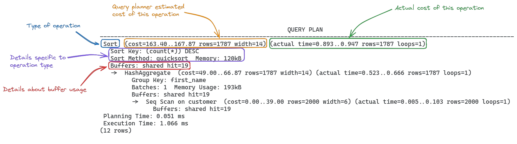
In this example, there are 3 operations: Sort which operates on the output of HashAggregate, which runs on the data read by the Seq Scan (sequential scan of the table).

In order to run, the Seq Scan first needs to read the table, then the HashAggregate groups by the first_name column and finally Sort brings the results in the desired order.
When an operation arrow -> appears on the same level as another one, their operations are executed in order from top to bottom. This new query plan shows such a sequence:
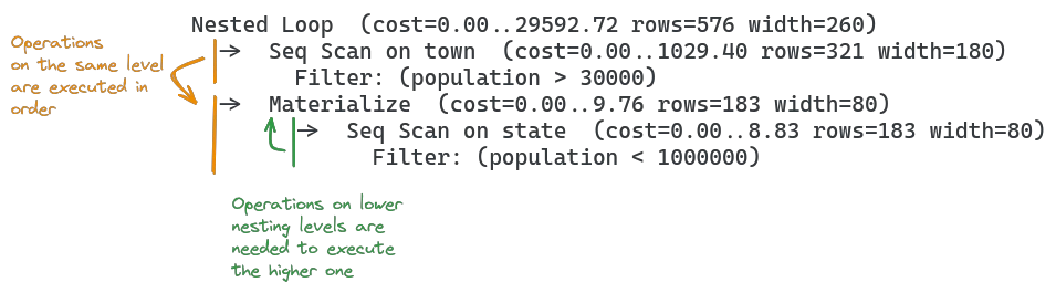
In the illustration above, the order operations are executed in would be:
Seq Scan on town, because it is first in orderMaterializeis next in order, but it depends onSeq Scan on state, so this runs secondFinally,
Materializecan run
Operations
Each operation in a query plan describes a specific task to process data. The most common operations for postgres are:
Seq Scan: Scans the entire table row by row; usually the slowest option.
Index Scan: Scans the table using an index; faster than a seq scan but can still involve table lookups.
Index Only Scan: Scans the index without accessing the table data; faster than an index scan.
Bitmap Index Scan: Uses a bitmap index for scanning, efficient for multiple conditions; slower than an index scan but faster than a seq scan.
Bitmap Heap Scan: Uses a bitmap to retrieve rows from the table; used with bitmap index scan, generally faster than a seq scan.
Tid Scan: Retrieves rows by their tuple IDs; very fast but rarely used directly.
Subquery Scan: Scans the result of a subquery as if it were a table; performance depends on the subquery complexity.
Values Scan: Scans a set of constant values; generally very fast.
CTE Scan: Scans the result of a Common Table Expression (CTE); performance varies with CTE complexity.
Function Scan: Scans the result of a set-returning function; performance depends on the function.
Nested Loop: Performs a nested-loop join between two tables; can be slow for large datasets without indexing.
Merge Join: Performs a merge join on sorted inputs; faster than a nested loop for large sorted datasets.
Hash Join: Uses a hash table to join two tables; generally fast, especially for large unsorted datasets.
Hash: Builds a hash table of the result set; used in hash joins and hash aggregates.
Append: Appends the results of multiple sub-plans; performance depends on the sub-plans.
Merge Append: Merges the results of multiple sub-plans while preserving order; useful for ordered results, slightly slower than append.
Recursive Union: Supports recursive queries, useful for hierarchical data; performance depends on recursion depth and dataset size.
Gather: Collects results from parallel worker processes; improves performance through parallelism.
Gather Merge: Merges sorted results from parallel worker processes; combines parallelism with order preservation, usually slower than gather.
Sort: Sorts the result set; can be slow for large datasets, especially without indexes.
Group: Groups the result set by one or more columns; typically used with aggregation functions, performance varies.
Aggregate: Performs aggregation functions like SUM or COUNT; performance varies based on dataset size.
HashAggregate: Performs aggregation using a hash table; efficient for large group-by operations.
Limit: Limits the number of rows returned; generally fast.
Unique: Removes duplicate rows; can be slow for large datasets without indexes.
Materialize: Stores intermediate results to avoid recomputation; useful for complex queries, can increase memory usage.
Which operations are chosen can differ wildly based on the data to be processed. Even if an index is available for an index scan for example, if a large portion of the table rows are estimated to be returned, the query planner may use a sequential scan to retrieve them instead, as that is likely faster (sequential i/o is faster for larger amounts of data, as random i/o typically has seek overhead).
Operation cost
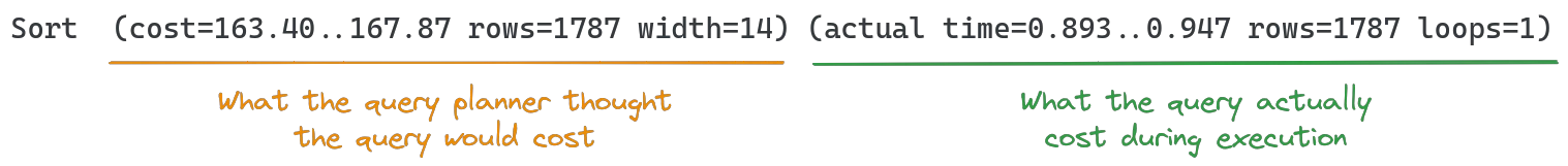
The cost of an operation is printed in brackets () and contains multiple fields with information. Each operation will have two different sets of cost information: The first is the estimate from the query planner, which it used to come up with the query plan (especially dependency operations). These will typically be close to the actual cost, as long as the table statistics are up to date. The second set of cost information shows the actual cost of running the query.
The estimated cost contains the following values:
cost: startup cost, followed by.., then total cost. The numbers are arbitrary and only useful relative to other cost numbers in the same query plan; lower values are better. Startup cost defines the estimated time to returning the first row, total cost the estimated time until returning the last row of the operation resultsrows: estimated number of rows returned from the operationwidth: estimated average size of each row (in bytes)
The actual cost contains similar, but slightly different values:
actual time: startup time, followed by.., then total time. Times are given in ms. Startup time is the time taken to returning the first row, total time is the time taken to return the last row of the operation results.rows: actual number of rows returned from the operationloops: number of times the operation ran
The last piece of information needed to understand query plan costs is that cost and actual time are treated differently. Consider this query plan:
 Sort (cost=163.40..167.87 rows=1787 width=14) (actual time=0.893..0.947 rows=1787 loops=1)
  Sort Key: (count(*)) DESC
  Sort Method: quicksort Memory: 120kB
  Buffers: shared hit=19
  -> HashAggregate (cost=49.00..66.87 rows=1787 width=14) (actual time=0.523..0.666 rows=1787 loops=1)
        Group Key: first_name
        Batches: 1 Memory Usage: 193kB
        Buffers: shared hit=19
        -> Seq Scan on customer (cost=0.00..39.00 rows=2000 width=6) (actual time=0.005..0.103 rows=2000 loops=1)
              Buffers: shared hit=19
 Planning Time: 0.051 ms
 Execution Time: 1.066 ms
The cost= values are not affected by the cost values of previous operations. For the actual time= values however, this is not true: The 0.103ms total time taken for the Seq Scan is part of the HashAggregate startup time of 0.523ms, because it had to wait for it to finish to process it's data. This means that the startup time for HashAggregate without the time spent waiting for the Seq Scan to finish was 0.42ms.
Operation details
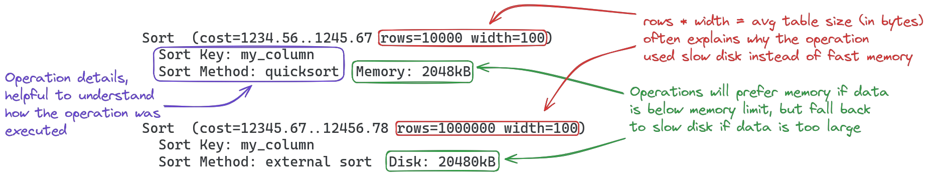
The format of the operation details is a range of key-value pairs, like Memory: 1024kB or Sort Key: age. The fields that are present depend on the operation and how it was executed. When debugging performance issues with a query, you are typically going to look for one of two keywords: Memory or Disk. Operations will prefer to use memory to run, but fall back to using the slower disk if the data does not fit into memory (specifically, the data + the memory the operation needs to run are larger than the work_mem limit specified in postgresql.conf).
If the Disk keyword is present in an operation's details, that may be a first indicator that something could be optimized in this operation. Why (and how) the disk was used depends on the operation and data it operated on, this is where the other operation details may come in handy to further understand what exactly was done in this step of the query plan.
It is important to understand that the actual memory used for each operation depends in various factors. The rows and width fields of the cost information will give you a rough hint how the total memory requirement was calculated, as rows * width = roughly size of table. This is not accurate however, as width represents the average size per row, so calculations will likely not be accurate. Operations also need memory to run themselves (for example to keep intermediate values in memory), so the actual needed amount may be slightly higher than the size of the table.
Buffers
The postgres server attempts to keep frequently used data in memory, (aka. in "buffer pools"). Query operations working on buffers are significantly faster than those involving disk i/o.
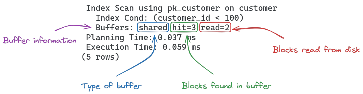
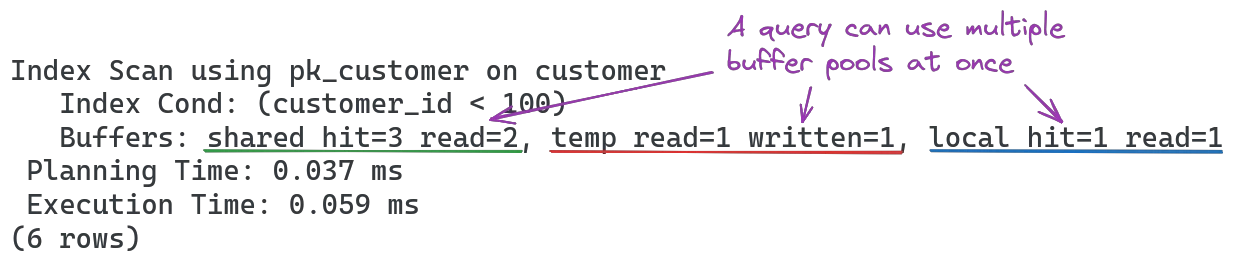
When talking about buffers, there are three kinds that a query may hit:
Shared: Most likely buffer to hit. Shared buffer is a memory pool that holds frequently used data from the entire server, to try and minimize the impact of common queries.
Local: Session-scoped cache, used for example by temporary table or views.
Temporary: Temporary files, like those used for external sorting or when flushing intermediate results to disk for large data sets.
A single operation can access multiple buffers at once. Each buffer can have up to four fields indicating how it was accessed:
hit: Blocks found in the buffer pool (memory cache)
read: Blocks that had to be read from disk into buffer pool
dirtied: Blocks that were modified in buffer pool, but did not need to be written to disk (yet)
written: Blocks written to disk
The amount of data for each of these fields is specified in "blocks"; these can be configured when setting up the PostgreSQL cluster and will default to 8kB. From a performance standpoint, the fields hit and dirtied are optimal for query execution speed, while read and written may indicate an optimization opportunity, either by increasing cache sizes, keeping the data in the relevant buffer pool for longer or decreasing the data to process in order to minimize blocks read from/written to disk.